In this blog post I will discuss how to implement Depth-first search (DFS) and Breadth-first search (BFS) in the functional programming language Haskell.
Before we get started by defining types for search problems and algorithms, let us import some useful library functions.
module Search where
import Data.List (find,nub)
import Data.Maybe (listToMaybe,mapMaybe)
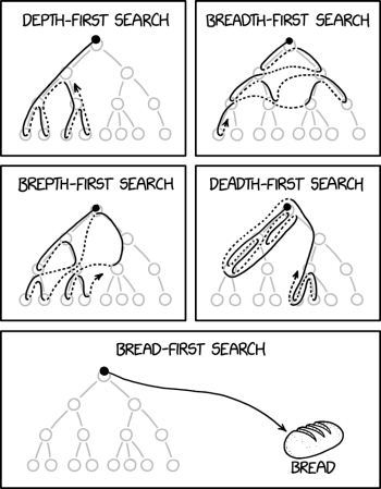
import Debug.Trace (trace)A classic way to show the difference between DFS and BFS uses binary trees:
But search problems and algorithms are more general than binary trees.
What is a search problem?
In general, a search problem is given by:
- a
startvalue where we begin our search, - an
expandmethod to compute possible new values, - a property
isDonetelling us whether a given value is or suffices as a goal.
data SearchProb a =
  SearchProb { start :: a
             , expand :: a -> [a]
             , isDone :: a -> Bool }
Here is a very simple search problem: How can we go from 23 to 42 by repeatedly adding 2 or 5?
findNumber :: SearchProb Int
findNumber = SearchProb
  { start = 23
  , expand = \n -> concat [ [ n+2, n+5] | n < 42 ]
  , isDone = (==42) }
In order to see what is happening and in which order, we use trace:
findNumber' :: SearchProb Int
findNumber' = SearchProb
  { start = 23
  , expand = \n -> trace (show n) concat [ [ n+2, n+5] | n < 42 ]
  , isDone = (==42) }
Another example: How can we move from (0,0) to (4,4) in a two-dimensional grid?
(Note that here we use trace again to print intermediate steps.)
grid :: SearchProb (Int,Int)
grid = SearchProb start expand isDone where
  start = (0,0)
  expand = \(x,y) -> trace (show (x,y)) $ [ (x+1,y) | x < 4 ] ++ [ (x,y+1) | y < 4 ]
  isDone = (== (4,4))
And another example, with a binary tree:
data BinaryTree a = Empty | Node a (BinaryTree a) (BinaryTree a) deriving (Show)

findInTree :: BinaryTree a -> (a -> Bool) -> SearchProb (BinaryTree a)
findInTree start isDone = SearchProb start subtrees treeIsDone where
  treeIsDone Empty        = False
  treeIsDone (Node x _ _) = isDone x
  subtrees Empty          = []
  subtrees (Node _ a b)   = [a, b]

exampleTree :: BinaryTree String
exampleTree = Node "Hay"
               (Node "Hay"
                 (Node "Hay" Empty Empty)
                 (Node "Needle A" Empty Empty))
               (Node "Needle B"
                 (Node "Hay" Empty Empty)
                 Empty)

findNeedle :: SearchProb (BinaryTree String)
findNeedle = findInTree exampleTree (("Needle" ==) . take 6)
What is a Search Algorithm?
Well, something that hopefully solves a search problem. So a search algorithm takes a search problem and then maybe returns a value:
type SearchAlgo a = SearchProb a -> Maybe aDFS and BFS in Haskell
dfs :: SearchAlgo a
dfs (SearchProb start expand isDone) = loop start where
  loop x | isDone x  = Just x
         | otherwise = listToMaybe $ mapMaybe loop (expand x)
To summarise the definition of loop: If the current x is what we wanted to find, then stop with Just x. Otherwise, apply the expand function to x and then map the loop function over this list.
Here it is crucial that Haskell is lazy: the resulting list expand x will not be fully evaluated before the loop function is called again.
Instead, loop will be applied to the first element of expand x and only if the result is Nothing the next element will be tried.
(By the way, this means dfs can work even if we have an infinitely branching search problem where expand x is an infinite list.)
BFS also uses a loop.
But crucially, the parameter of loop in bfs is a list xs instead of a single point x.
bfs :: SearchAlgo a
bfs (SearchProb start expand isDone) = loop [start] where
  loop xs | any isDone xs = find isDone xs
          | otherwise     = loop (concatMap expand xs)
DFS and BFS also differ in which function is mapped:
- In DFS we map
loopover the result ofexpand x. - In BFS we map
expandover allxsand apply loop to the result.
Examples
λ> dfs findNumber
Just 42
λ> bfs findNumber
Just 42
Well, that is not very informative, both algorithms find the same result of course.
But the way they find it is different, and we can see that if we use findNumer' which prints intermediate steps.
λ> dfs findNumber'
23
25
27
29
31
33
35
37
39
41
43
46
44
Just 42
λ> bfs findNumber'
23
25
28
27
30
30
33
29
32
32
35
32
35
35
38
31
34
34
37
Just 42
Looking at the grid example we can also see that our bfs implementations is very inefficient.
It visits many fields in the grid multiple times.
λ> dfs grid
(0,0)
(1,0)
(2,0)
(3,0)
(4,0)
(4,1)
(4,2)
(4,3)
Just (4,4)
λ> bfs grid
(0,0)
(1,0)
(0,1)
(2,0)
(1,1)
(1,1)
(0,2)
(3,0)
(2,1)
(2,1)
(1,2)
(2,1)
(1,2)
(1,2)
(0,3)
(4,0)
(3,1)
(3,1)
(2,2)
(3,1)
(2,2)
(2,2)
(1,3)
(3,1)
(2,2)
(2,2)
(1,3)
(2,2)
(1,3)
(1,3)
(0,4)
(4,1)
(4,1)
(3,2)
(4,1)
(3,2)
(3,2)
(2,3)
(4,1)
(3,2)
(3,2)
(2,3)
(3,2)
(2,3)
(2,3)
(1,4)
(4,1)
(3,2)
(3,2)
(2,3)
(3,2)
(2,3)
(2,3)
(1,4)
(3,2)
(2,3)
(2,3)
(1,4)
(2,3)
(1,4)
(1,4)
(4,2)
(4,2)
(4,2)
(3,3)
(4,2)
(4,2)
(3,3)
(4,2)
(3,3)
(3,3)
(2,4)
(4,2)
(4,2)
(3,3)
(4,2)
(3,3)
(3,3)
(2,4)
(4,2)
(3,3)
(3,3)
(2,4)
(3,3)
(2,4)
(2,4)
(4,2)
(4,2)
(3,3)
(4,2)
(3,3)
(3,3)
(2,4)
(4,2)
(3,3)
(3,3)
(2,4)
(3,3)
(2,4)
(2,4)
(4,2)
(3,3)
(3,3)
(2,4)
(3,3)
(2,4)
(2,4)
(3,3)
(2,4)
(2,4)
(2,4)
(4,3)
Just (4,4)
We can improve this a bit with a nub to remove duplicates from the list passed to "loop".
slightlyBetterBfs :: Eq a=> SearchAlgo a
slightlyBetterBfs (SearchProb start expand isDone) = loop [start] where
  loop xs | any isDone xs = find isDone xs
          | otherwise     = loop (nub $ concatMap expand xs)
λ> slightlyBetterBfs grid
(0,0)
(1,0)
(0,1)
(2,0)
(1,1)
(0,2)
(3,0)
(2,1)
(1,2)
(0,3)
(4,0)
(3,1)
(2,2)
(1,3)
(0,4)
(4,1)
(3,2)
(2,3)
(1,4)
(4,2)
(3,3)
(2,4)
(4,3)
Just (4,4)Getting back to binary trees, we can see that DFS and BFS will find different answers:
λ> dfs findNeedle
Just (Node "Needle A" Empty Empty)
λ> bfs findNeedle
Just (Node "Needle B" (Node "Hay" Empty Empty) (Node "Hay" Empty Empty))
Finally, it is very easy to define search problems on which DFS will run forever.
λ> dfs (SearchProb (1::Int) (\n -> [n*3,n*2]) even)
^CInterrupted.
λ> bfs (SearchProb (1::Int) (\n -> [n*3,n*2]) even)
Just 2
The order in which expand generates new values also matters for the result.
λ> bfs (1::Int) (\n -> [n*3,n*2]) (\n -> even n && n > 200)
Just 486
λ> bfs (1::Int) (\n -> [n*2,n*3]) (\n -> even n && n > 200)
Just 216

λ> dfs (1::Int) (\n -> [n*2,n*3]) (\n -> even n && n > 200)
Just 256
λ> dfs (1::Int) (\n -> [n*3,n*2]) (\n -> even n && n > 200)
^CInterrupted.